Natural Language Processing (NLP) with Deep Learning

Introduction

Natural Language Processing is one of the many branches of computer science that enables the computer’s ability to understand languages.

This was my submission for a Kaggle Competition, “Natural Language Processing with Disaster Tweets“.

The objective is to determine if a certain tweet is referring to an actual disaster or not.

This is a brief blog post on how to use deep learning to predict if the tweets are talking about actual disasters.

I used Google Colab for my project to use their GPU to run the code faster.

Disclaimer: This is a code which I have written and it may or may not be the most efficient method.
If you have any suggestions or feedback, I am willing to receive constructive feedback.

Importing relevant libraries

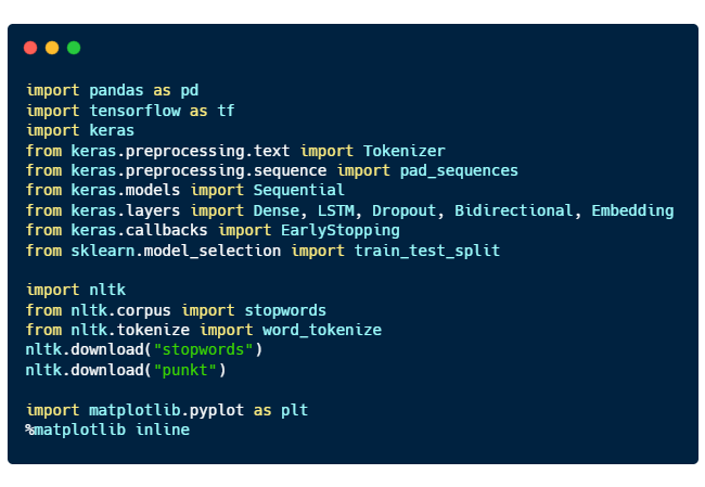
Here are the purposes of each libraries imported:

pandas for processing data
tensorflow and keras for deep learning
nltk, natural language toolkit for natural language processing
matplotlib for plotting graphs

Reading the csv file

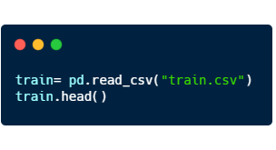
Using pandas, we can read the csv file.
“train.head()” will return the first 5 rows of the dataset.

Here’s a sample of what is inside

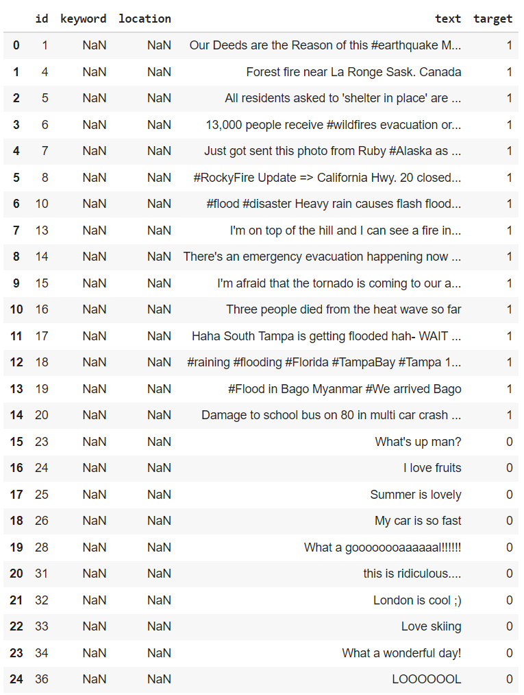
From here, we can see that disaster tweets are denoted by the target value of “1”, and if they are not, they are assigned the target value “0”.

Data Cleaning

As we can see from the figure above, the data can contain a lot of not very useful information such as the columns “keyword” and “location” as they are mostly empty values.

So before we give the computer to understand what we are saying, we have to clean up the mess in the data.

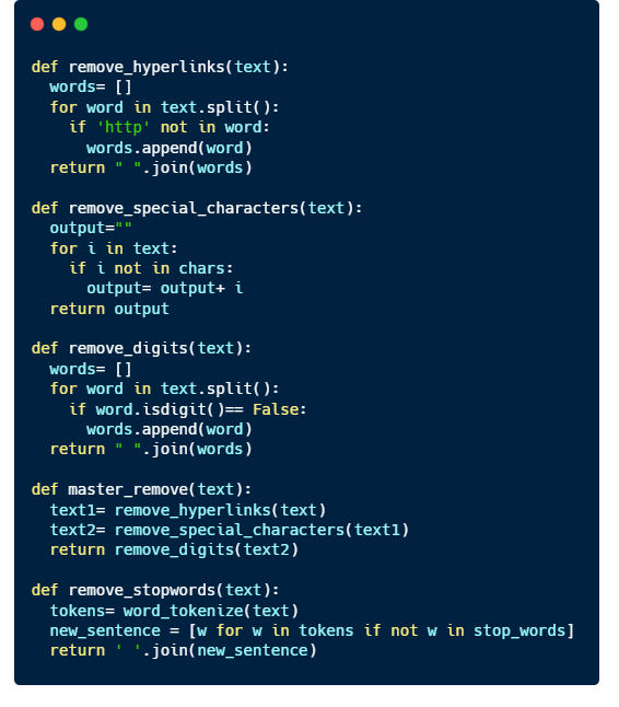
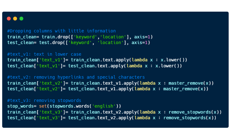
We will do just a simple data cleaning which consists of

Dropping the columns “keyword” and “location”.
Making all text to be in lower case
Removing hyperlinks and special characters (#, @, %, … )
Removing stopwords.

Before we move on, here’s a very brief introduction to what are stopwords.
Stopwords are words that does not contain much information.
They are mostly pronouns, prepositions, and conjunctions.
Here are some samples of stopwords:

{'again', 'doing', 'off', 'were', 'these', 'and', 'so', 'are', 'as', 'who', 'has', 'this', 'yourself', 'me'}

Let’s write some functions to make our data cleaning a little bit easier 🙂

Implement the code to the training and test datasets.

Here’s a sample of how an entry looks like after data cleaning.

id                            38
text       Was in NYC last week!  #original text

text_v1    was in nyc last week!  #lower case
text_v2     was in nyc last week  #special character removed
text_v3            nyc last week  #stopwords removed
target                         0

Tokenization

Now that we have our data cleaned, we can now give it to the computer to do the ‘learning’.

Well not exactly.

Computers understand numbers better than they understand English, so we have to somehow convert our texts to numbers. That’s when we have to do Tokenization.

How it works.

You can think of tokenization as a 1-1 function.
There exists one and ONLY one number that correlates to one English word.

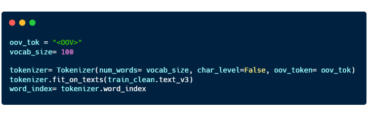
In the code above, we are using the words from “train_clean.text_v3” to form a dictionary consisting of English words and its corresponding numerical value.

“oov_tok” is a token that is assigned to words that are out-of-vocabulary.
“vocab_size” is the number of tokenized words you want to keep. Only the most common words are kept.
“char_level” is put as False. If True, every character will be treated as a token.

Here’s a sample of what is in the “word_index”:

{..., 'video': 14,
 'emergency': 15,
 'disaster': 16,
 'police': 17, ... }

train_test_split

When training the model, we have to divide the training dataset into 2 separate two groups of data. Training data and Validation data.

You can think of machine learning/ deep learning like drawing a best fit curve on a scatterplot. With just the training dataset, you can definitely draw a curve passing through all the points, and you obtain a model with very high accuracy on a training dataset as your mean squared error is zero.

However, data in real world are subjected to errors and thus, the model that you developed may not reflect the general trend that occurs in reality.

This leads to overfitting and to avoid this from happening, we have to have a validation dataset to ‘check’ to ensure that the model is able to be applied to a larger context.

Here’s the code for “train_test_split”:

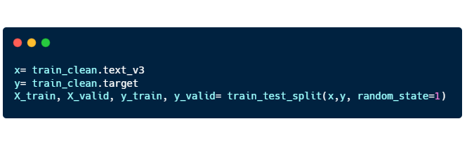
X_train, X_valid: “text_v3” training and validation
Y_train, Y_valid: “target” training and validation

Padding

The final step we have to do before we train the model is padding.

Language consist of sentences with varying lengths, but computers can only learn when the input is of the same length for all sentences. So we have to fill in the gaps for shorter sentences by padding them.

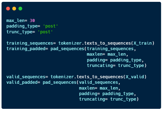
“max_len”: maximum length of the sentence
“padding_type” : sentences will be padded at the end
“trunc_type”: sentences longer than max_len will be cut short from the back

Building a model

The model consists of 4 layers: 2 Bidirectional LSTM layers and 2 Dense layers.

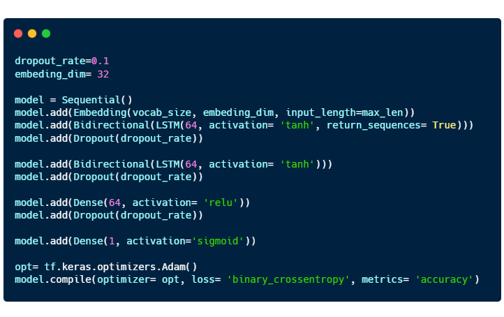
Embedding is a way to represent words using dense vectors in a continuous vector space.
Activation functions for Bidirectional LSTM and Dense layer are “tanh” and “relu” respectively.
The last Dense layer uses a “sigmoid” function as this is a classification problem.
“Adam” optimizer is used.

“epoch” : the number of passes of the entire training dataset the machine learning algorithm has completed
“early_stopping” is implemented so that the training stops when the maximum validation accuracy (“val_accuracy”) is attained.

Here’s the result of the trained model.

60/60 [==============================] - 0s 6ms/step - loss: 0.5470 - accuracy: 0.7269
[0.5469951629638672, 0.7268907427787781]

Not bad, but definitely can be improved 😀